Topic 4c: Solving Ordinary Differential Equations
Contents
Topic 4c: Solving Ordinary Differential Equations#
import numpy as np
import matplotlib.pyplot as plt
Solving equations numerically is a useful skill, but was not terribly difficult to code ourselves. The situation quickly escalates when we move from solving algebriac equations to differential equations. In principle we can still do it outselves but the job is definiely more complex.
We will again take an experimental approach, we will start with a problem we know how to solve and try to see what is happening. Let’s take the case of the 1d harmonic oscilator
\(\ddot x + \gamma \dot x + \omega_0^2 x = 0\)
The way that python deals with these equations is to reduce them to a coupled set of first order equations. This is perhaps the part that is more annoying, “Why can’t I just write the equation I want to solve???”. We can try to work out the advantages later, but for now you just have to deal with it.
In this case, we define it as follows:
\(\dot x = v\)
and
\(\dot v = -\gamma v - \omega_0^2 x\)
So we have two variables, position \(x\) and velocity \(v\), that both evolve according to first order ODEs but their evolution is coupled (\(\dot v\) depends on \(x\))
Now we define a function that, given a v and x, returns these derivatives:
def derivative(X,t,gamma=1,omega_0=1): ## X is the array [x,v]
        ## notice that we need to use t as an argument even though we don't use it
    return np.array([X[1],-gamma*X[1]-omega_0**2*X[0]]) ## return the array dot X defined by our equation
from scipy import integrate
We have defined the equation. We now need to know the initial conditions and where we are solving this (this is numerical, so we have to pick some finite amount of time):
t_R=np.linspace(0,10,100) # range of time we want to solve
X0=[3.,0]     #initial conditions
Now we use the basic ODE integrator in scipy
sol1=integrate.odeint(derivative,X0,t_R) #syntax - odeint(derivative,initial conditon, time)
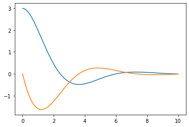
plt.plot(t_R,sol1[:,0])  # returns solution for X at each point in time  sol[:,0] is x(t)
plt.plot(t_R,sol1[:,1])  # returns solution for X at each point in time  sol[:,1] is v(t)
plt.show()
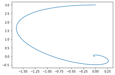
One way to think about what our odeint is doing is moving our solution through “phase space”, namely (v,x). Time allows us to define a path through this space but we can think of the results as just a curve as so:
plt.plot(sol1[:,1],sol1[:,0])  #phase space plot
plt.show()
I secretly planned ahead when I derived my derivative function. Because odtint takes a function as input, you can pass any of the variabels that the function defines. This goes under the “args” option, where we pass this assition infomration
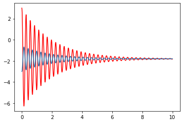
sol2=integrate.odeint(derivative,X0,t_R,args=(2,20)) # now passing gamma=2 and omega_0=20
plt.plot(t_R,sol2[:,0])  # returns solution for X at each point in time  sol[:,0] is x(t)
#plt.plot(t_R,sol2[:,1])  # returns solution for X at each point in time  sol[:,1] is v(t)
plt.show()
Now let’s see how well it is tracking the exact solution. To make this extra easy, let’s take \(\gamma=0\) so that our solution should be $\(x(t) = 3 \cos(\omega_0 t)\)$
sol3=integrate.odeint(derivative,X0,t_R,args=(0,20)) # now passing gamma=0 and omega_0=20
plt.plot(t_R,sol3[:,0])  # returns solution for X at each point in time  sol[:,0] is x(t)
#plt.plot(t_R,3*np.cos(20*t_R))  # returns solution for X at each point in time  sol[:,1] is v(t)
plt.show()
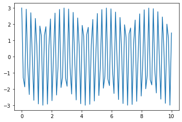
At first sight, our solution clearly looks wrong. Our exact solution is supposed to be a pure cosine and it looks like it is the produce of two oscilations. But this isn’t what is happening, because the error is actually pretty small:
plt.plot(t_R,sol3[:,0]-3*np.cos(20*t_R))  # returns solution for X at each point in time  sol[:,0] is x(t)
#plt.plot(t_R,3*np.cos(20*t_R))  # returns solution for X at each point in time  sol[:,1] is v(t)
plt.show()
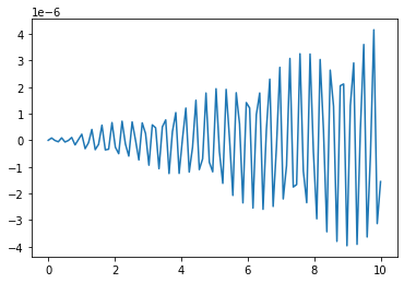
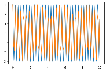
Instead, we have encountered the aliasing. This is what happens whe you sample an oscilation at too low a frequency. Basically what is happening is that we are sampling our function at too slow a rate to resolve the actual oscilation properly so what comes out is something that looks like a lower frequency. We can see that just by increasing the spacing between the points.
t_n=np.linspace(0,10,1000)
plt.plot(t_n,3*np.cos(20*t_n))
plt.plot(t_R,3*np.cos(20*t_R))
[<matplotlib.lines.Line2D at 0x11a1ae850>]
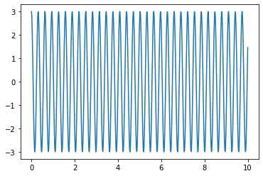
Knowing that, we can do the same for our solution:
sol3n=integrate.odeint(derivative,X0,t_n,args=(0,20)) # now passing gamma=0 and omega_0=20
plt.plot(t_n,sol3n[:,0])  # returns solution for X at each point in time  sol[:,0] is x(t)
#plt.plot(t_R,3*np.cos(20*t_R))  # returns solution for X at each point in time  sol[:,1] is v(t)
plt.show()
However this doesn’t improve our error, because this is just the points we are asking it to return a solution:
plt.plot(t_R,np.abs(sol3[:,0]-3*np.cos(20*t_R)),color='red')
plt.plot(t_n,np.abs(sol3n[:,0]-3*np.cos(20*t_n)))
plt.yscale('log')
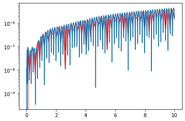
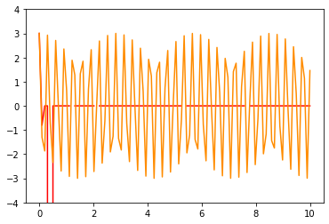
The sampling time is presumably a parameter in the function itself:
sol5=integrate.odeint(derivative,X0,t_R,args=(0,20),mxstep=47)
sol6=integrate.odeint(derivative,X0,t_R,args=(0,20),mxstep=100)
/opt/anaconda3/lib/python3.9/site-packages/scipy/integrate/odepack.py:247: ODEintWarning: Excess work done on this call (perhaps wrong Dfun type). Run with full_output = 1 to get quantitative information.
  warnings.warn(warning_msg, ODEintWarning)
plt.plot(t_R,sol5[:,0],color='red')
plt.plot(t_R,sol6[:,0],color='darkorange')
#plt.plot(t_R,sol3[:,0])
plt.ylim(-4,4)
(-4.0, 4.0)
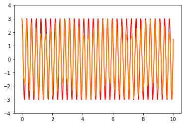
t_F=np.linspace(0,10,10000) # range of time we want to solve
sol7=integrate.odeint(derivative,X0,t_F,args=(0,20),mxstep=20)  # Using finer spacing but fewer interal steps
plt.plot(t_F,sol7[:,0],color='red')
plt.plot(t_R,sol6[:,0],color='darkorange')
#plt.plot(t_R,sol3[:,0])
plt.ylim(-4,4)
(-4.0, 4.0)
plt.plot(t_F,np.abs(sol7[:,0]-3*np.cos(20*t_F)),color='red')
plt.plot(t_R,np.abs(sol3[:,0]-3*np.cos(20*t_R)))
plt.yscale('log')
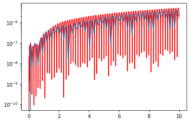
So we see that all that happened in some sense is that if we take in external time-grid to be finer, we don’t need as many interal steps. However, that has not explained the weird behavior with the error.
If we go and read the documentation, we find that our problem is that ODEint is making a lot of decisions for us. Changing these parameters is not helping because ODE already tried to optimize the problem.
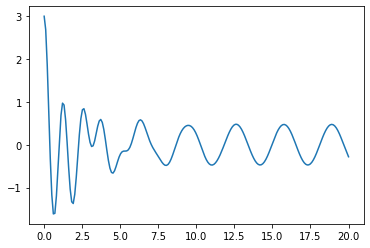
Time-dependent coefficients, External Force#
def D_time(X,t,gamma=1,omega_0=5,Fext=10,wext=2): ## X is the array [x,v]
        ## notice that we need to use t as an argument even though we don't use it
    return [X[1],-gamma*X[1]-omega_0**2*X[0]+Fext*np.cos(wext*t)] ## return the array dot X defined by our equation
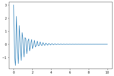
t_T=np.linspace(0,20,200)
solT_1=integrate.odeint(D_time,X0,t_T) # now passing gamma=0 and omega_0=20
plt.plot(t_T,solT_1[:,0])
[<matplotlib.lines.Line2D at 0x11a2c22b0>]
Coupled ODEs#
Now we want to consider the problem of coupled harmonic oscilators, obeying the equation: $\(\ddot x +\gamma_x \dot x + \omega_x^2 (x-y) = 0\)\( \)\(\ddot y +\gamma_y \dot y + \omega_y^2 (y-x) = 0\)$
def D_coupled(X,t,gamma_x=1,omega_x=1,gamma_y=1,omega_y=1): ## X is the array [x,v]
        ## notice that we need to use t as an argument even though we don't use it
    return [X[1],-gamma_x*X[1]-omega_x**2*(X[0]-X[2]),X[3],-gamma_y*X[3]-omega_y**2*(X[2]-X[0])] ## return the array dot X defined by our equation
t_R=np.linspace(0,10,100) # range of time we want to solve
XC_0=[3.,0,-3.,0]
solC_1=integrate.odeint(D_coupled,XC_0,t_n,args=(1,20,1,10))
plt.plot(t_n,solC_1[:,0],color='red')
plt.plot(t_n,solC_1[:,2])
[<matplotlib.lines.Line2D at 0x119e0a7f0>]